Geomagnetism

Magnetic Field Model MF6

Satellites in low-Earth orbit (LEO) provide the most effective means of mapping the long wavelengths of the magnetic field caused by the magnetization of the Earth's crust. The first global magnetic anomaly maps were produced from POGO (1960s) and Magsat (1979) satellite measurements. A breakthrough in resolution and accuracy was achieved with the CHAMP satellite, launched in July 2000. Apart from an order of magnitude improvement in magnetometer accuracy, CHAMP was designed to remain in LEO for many years, leading to excellent spatial coverage. The MF6 model was produced using a new scalar data product from the latest three years of measurements from the CHAMP flux-gate magnetometer. The modeling methodology remained largly unchanged from the previous version MF5. MF6 resolves the crustal magnetic field to spherical harmonic degree 120, corresponding to length scales down to 333 km. The MF6 model is the first satellite-based magnetic model to resolve the direction of oceanic magnetic lineations, revealing the age structure of oceanic crust (Fig. 1).

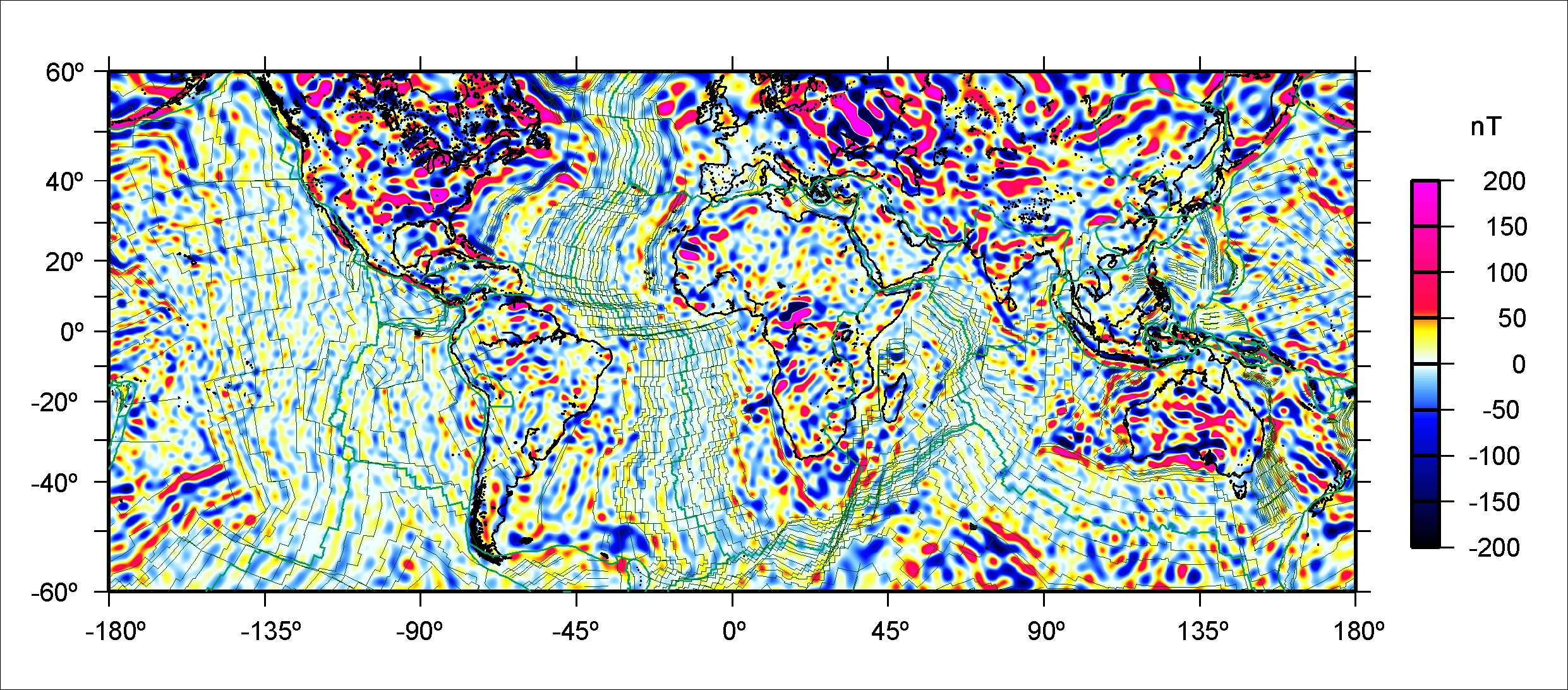
Fig.1: (click to enlarge) Fig. 1: Vertical component of the MF6 crustal magnetic field at the Earth surface, overlain with the isochrons of an ocean-age model inferred from independent marine and aeromagnetic data by Muller et al. (2007) and plate boundaries by Bird (2003).

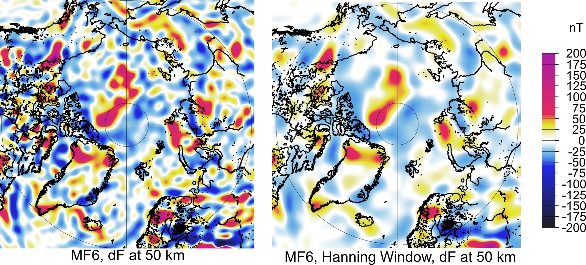
A cautionary note on "ringing" in satellite crustal maps: When displayed as maps at the Earth's surface, the satellite-based maps of the crustal magnetic field look "bubbly". This is not due to noise. The crustal field has a very flat (white) power spectrum at long wavelengths. A sharp cut-off at a certain spherical harmonic degree in the wavenumber domain leads to ringing in the space domain (the bubbles). In the case of MF6 this was mitigated somewhat by rolling off the power from degree 120 to degree 130, but that unfortunately does not make enough of a difference.

To completely get rid of the bubbliness one can apply a Hanning Window in the wavenumber domain, but at the cost of a significant loss in small-scale features (see Figure 2). As a general recommendation, one should use the un-fitered version (sharp cutoff) when substituting a long wavelength satellite model into a regional magnetic compilation of marine or aeromagnetic measurements, and the Hanning-windowed version when displaying the satellite model stand-alone. The table of products below includes Hanning-filtered versions of the grids of the anomaly of the total intensity at ellipsoid and 50 km altitude.

Fig.2: (click to enlarge) Fig. 2: Demonstration of the effect of the Hanning window. The left image shows the anomaly of the total intensity (dT) at 50 km altitude as given by MF6 with a sharp cutoff in the degree-band 120-130. The right image shows the result after applying a Hanning window to the MF6 spherical harmonic coefficients.

Available MF6 Downloads
	Type	Format	Mbyte	Ref. Radius	Contents
	SH coefficients	ASCII Table	0.2	6371.2 km	MF6 Model spherical harmonic coefficients (Schmid semi-normalized, as usual)
	Poster	PDF	13	WGS84	MF6 model poster at AGU conference, San Francisco, 2007
	Article	PDF	4.8		Sixth generation lithospheric magnetic field model from CHAMP satellite magnetic measurements
	Graphic	PDF	1.7	WGS84	Image of vertical component (Z) at WGS84 ellipsoid altitude.
	Listing	ZIP	42	WGS84	MF6_Z_0.xyz.gz 6 arc minute ascii grid of vertical component (Z) at WGS84 ellipsoid altitude.
	Graphic	PDF	1.8	WGS84	Image of the anomaly of total intensity at WGS84 ellipsoid altitude.
	Listing	ZIP	6	WGS84	MF6_dT_0.xyz.gz 15 arc minute ascii grid of the anomaly of total intensity at WGS84 ellipsoid altitude.
	Listing	ZIP	24	WGS84	MF6_dT_0_Hanning.xyz.gz 7.5 arc minute ascii grid of the anomaly of total intensity at WGS84 ellipsoid altitude, after applying a Hanning window to the MF6 coefficients.
	Listing	ZIP	24	WGS84 + 50 km	MF6_dT_50.xyz.gz 7.5 arc minute ascii grid of the anomaly of total intensity at 50 km altitude above the WGS84 ellipsoid.
	Listing	ZIP	24	WGS84 + 50 km	MF6_dT_50_Hanning.xyz.gz 7.5 arc minute ascii grid of the anomaly of total intensity at 50 km altitude above the WGS84 ellipsoid, after applying a Hanning window to the MF6 coefficients.
	Graphic	PDF	1.5	WGS84 + 350 km	Image of the anomaly of total intensity at 350 km altitude.
	Listing	ZIP	4	WGS84 + 350 km	MF6_dT_350.xyz.gz 15 arc minute ascii grid of the anomaly of total intensity at 350 km altitude.
	Video	MPEG	50	WGS84 + 50 km	MF6_Z_50.mpg Rotating globe animation of the vertical component of the crustal field at 50 km altitude.

2009-Oct-24, Stefan Maus